4주차 과제

11 분 소요

import pandas as pd
import numpy as np
import matplotlib.pyplot as plt
from sklearn.model_selection import train_test_split
from sklearn.preprocessing import MinMaxScaler
from sklearn.datasets import make_classification
from sklearn.neighbors import KNeighborsClassifier
from sklearn import metrics

1. 가상의 학생 성적 데이터를 활용한 데이터 전처리 과정을 구현해보세요.

가상의 학생 성적 데이터가 제공되지 않았으므로 가상의 학생 성적 데이터를 먼저 만들어 주어야한다.
가상 학생 성적 데이터를 만들기 위한 조건
1. 데이터 전처리 과정에서 결측치를 처리하는 과정을 구현해보기 위해서 결측치 즉, np.nan이 포함된 데이터를 만들고자 하였다.
2. 데이터 이상치를 확인하고 제거해보는 것을 구현하기 위해 성적이 0 ~ 100 사이가 아닌 값을 넣고자 하였다. 간단하게 (-1 혹은 101로 처리)
3. 2번 문제를 풀이하기 위해 100개의 데이터로 만들어보았다.

# 시드 설정
np.random.seed(42)

# 데이터 개수 설정
num_students = 100

# 학생 ID 생성
student_ids = np.arange(1, num_students + 1)

# 학생 나이 설정
ages = np.random.randint(17, 20, size=num_students)

# 학생 성별 설정
genders = np.random.choice(['Male', 'Female'], size=num_students)

# 학생 과목 점수 설정
math = np.random.randint(0, 101, size=num_students)
english = np.random.randint(0, 101, size=num_students)
science = np.random.randint(0, 101, size=num_students)

# DataFrame 생성
df = pd.DataFrame({
    'Student_ID': student_ids,
    'Age': ages,
    'Gender': genders,
    'Math': math,
    'English': english,
    'Science': science
})

# 결측치 추가
for col in ['Age', 'Math', 'English', 'Science']:
  nan_indices = np.random.choice(df.index, size=int(num_students * 0.1), replace=False)
  df.loc[nan_indices, col] = np.nan

# 이상치 추가
for col in ['Math', 'English', 'Science']:
  outlier_indices = np.random.choice(df.index, size=int(num_students * 0.1), replace=False)
  df.loc[outlier_indices, col] = np.random.choice([-1, 101])

df

	Student_ID	Age	Gender	Math	English	Science
0	1	19.0	Female	91.0	15.0	32.0
1	2	17.0	Female	88.0	89.0	66.0
2	3	19.0	Female	61.0	59.0	101.0
3	4	19.0	Male	96.0	NaN	24.0
4	5	17.0	Male	0.0	0.0	94.0
...	...	...	...	...	...	...
95	96	17.0	Female	101.0	96.0	89.0
96	97	17.0	Male	101.0	62.0	61.0
97	98	19.0	Female	41.0	84.0	101.0
98	99	17.0	Female	98.0	31.0	8.0
99	100	17.0	Male	NaN	NaN	11.0

100 rows × 6 columns

# 결측치 확인

nan_df = df[df.isna().any(axis=1)]
nan_df

	Student_ID	Age	Gender	Math	English	Science
3	4	19.0	Male	96.0	NaN	24.0
5	6	NaN	Male	26.0	47.0	53.0
6	7	19.0	Male	61.0	11.0	NaN
8	9	19.0	Male	2.0	36.0	NaN
14	15	NaN	Male	36.0	79.0	65.0
20	21	NaN	Female	NaN	23.0	101.0
24	25	17.0	Female	51.0	37.0	NaN
32	33	18.0	Female	NaN	81.0	59.0
41	42	19.0	Male	100.0	NaN	13.0
42	43	19.0	Male	95.0	32.0	NaN
49	50	NaN	Male	NaN	66.0	86.0
50	51	18.0	Male	31.0	NaN	62.0
51	52	17.0	Male	69.0	NaN	85.0
53	54	17.0	Female	NaN	75.0	24.0
54	55	NaN	Female	54.0	58.0	57.0
63	64	18.0	Male	NaN	26.0	41.0
65	66	18.0	Female	15.0	NaN	14.0
67	68	NaN	Male	72.0	96.0	59.0
71	72	NaN	Male	101.0	68.0	52.0
73	74	18.0	Male	NaN	47.0	4.0
74	75	18.0	Female	58.0	18.0	NaN
75	76	18.0	Male	101.0	NaN	5.0
77	78	19.0	Male	89.0	NaN	93.0
78	79	19.0	Male	66.0	-1.0	NaN
81	82	NaN	Female	95.0	NaN	39.0
82	83	18.0	Female	NaN	29.0	51.0
83	84	NaN	Female	51.0	92.0	101.0
86	87	NaN	Male	101.0	98.0	18.0
87	88	17.0	Male	NaN	36.0	NaN
91	92	17.0	Female	56.0	NaN	57.0
99	100	17.0	Male	NaN	NaN	11.0

# 이상치 확인

outlier_df = df[(df['Math'] < 0) | (df['English'] < 0) | (df['Science'] < 0) | (df['Math'] > 100) | (df['English'] > 100) | (df['Science'] > 100)]
outlier_df

	Student_ID	Age	Gender	Math	English	Science
2	3	19.0	Female	61.0	59.0	101.0
15	16	17.0	Female	96.0	-1.0	101.0
20	21	NaN	Female	NaN	23.0	101.0
26	27	17.0	Male	101.0	98.0	25.0
27	28	19.0	Female	51.0	-1.0	98.0
29	30	19.0	Male	38.0	24.0	101.0
31	32	19.0	Female	2.0	17.0	101.0
36	37	19.0	Male	1.0	79.0	101.0
38	39	17.0	Male	91.0	-1.0	64.0
40	41	17.0	Female	86.0	-1.0	101.0
47	48	17.0	Female	52.0	7.0	101.0
55	56	19.0	Female	74.0	-1.0	62.0
57	58	17.0	Male	101.0	29.0	21.0
59	60	19.0	Female	101.0	50.0	57.0
60	61	18.0	Male	68.0	-1.0	85.0
61	62	17.0	Male	101.0	7.0	48.0
71	72	NaN	Male	101.0	68.0	52.0
75	76	18.0	Male	101.0	NaN	5.0
78	79	19.0	Male	66.0	-1.0	NaN
79	80	18.0	Male	18.0	-1.0	98.0
83	84	NaN	Female	51.0	92.0	101.0
86	87	NaN	Male	101.0	98.0	18.0
89	90	17.0	Female	101.0	-1.0	18.0
92	93	17.0	Female	88.0	-1.0	54.0
95	96	17.0	Female	101.0	96.0	89.0
96	97	17.0	Male	101.0	62.0	61.0
97	98	19.0	Female	41.0	84.0	101.0

이상치 처리 : 이상치가 결측치 보간에 영향을 줄 수 있으므로 이상치 먼저 처리한다.</br> 이상치에서 -1은 np.nan이라고 판단하고 np.nan으로 바꿔넣고 101은 완전 이상치라 판단하고 제거해보았다.

df = df[(df['Math'] <= 100) & (df['Age'] <= 100) & (df['Science'] <= 100)]
df.replace(-1, np.nan, inplace=True)
df

<ipython-input-51-c5d88ba489df>:2: SettingWithCopyWarning: 
A value is trying to be set on a copy of a slice from a DataFrame

See the caveats in the documentation: https://pandas.pydata.org/pandas-docs/stable/user_guide/indexing.html#returning-a-view-versus-a-copy
  df.replace(-1, np.nan, inplace=True)

	Student_ID	Age	Gender	Math	English	Science
0	1	19.0	Female	91.0	15.0	32.0
1	2	17.0	Female	88.0	89.0	66.0
3	4	19.0	Male	96.0	NaN	24.0
4	5	17.0	Male	0.0	0.0	94.0
7	8	18.0	Female	76.0	68.0	66.0
...	...	...	...	...	...	...
91	92	17.0	Female	56.0	NaN	57.0
92	93	17.0	Female	88.0	NaN	54.0
93	94	19.0	Female	49.0	98.0	89.0
94	95	17.0	Female	22.0	59.0	100.0
98	99	17.0	Female	98.0	31.0	8.0

61 rows × 6 columns

결측값 처리 : 데이터 확인 결과 의도치 않게 Age가 결측치인 것들은 점수 들 중 하나가 101 이상치로 나와 다 제거 되었다. 하지만 Age의 값이 np.nan일 경우 중앙값으로 대체하는 코드를 첨부한다.

df.loc[:, 'Age'] = df['Age'].fillna(df['Age'].median())
df.loc[:, 'Math'] = df['Math'].fillna(df['Math'].mean())
df.loc[:, 'English'] = df['English'].fillna(df['English'].mean())
df.loc[:, 'Science'] = df['Science'].fillna(df['Science'].mean())

df

	Student_ID	Age	Gender	Math	English	Science
0	1	19.0	Female	91.0	15.0	32.0
1	2	17.0	Female	88.0	89.0	66.0
3	4	19.0	Male	96.0	47.0	24.0
4	5	17.0	Male	0.0	0.0	94.0
7	8	18.0	Female	76.0	68.0	66.0
...	...	...	...	...	...	...
91	92	17.0	Female	56.0	47.0	57.0
92	93	17.0	Female	88.0	47.0	54.0
93	94	19.0	Female	49.0	98.0	89.0
94	95	17.0	Female	22.0	59.0	100.0
98	99	17.0	Female	98.0	31.0	8.0

61 rows × 6 columns

데이터 정규화 : MinMaxScale을 이용해 정규화하였다.

scaler = MinMaxScaler()

df[['Age', 'Math', 'English', 'Science']] = scaler.fit_transform(df[['Age', 'Math', 'English', 'Science']])
df

<ipython-input-53-1f2fd14bdd15>:3: SettingWithCopyWarning: 
A value is trying to be set on a copy of a slice from a DataFrame.
Try using .loc[row_indexer,col_indexer] = value instead

See the caveats in the documentation: https://pandas.pydata.org/pandas-docs/stable/user_guide/indexing.html#returning-a-view-versus-a-copy
  df[['Age', 'Math', 'English', 'Science']] = scaler.fit_transform(df[['Age', 'Math', 'English', 'Science']])

	Student_ID	Age	Gender	Math	English	Science
0	1	1.0	Female	0.91	0.151515	0.313131
1	2	0.0	Female	0.88	0.898990	0.656566
3	4	1.0	Male	0.96	0.474747	0.232323
4	5	0.0	Male	0.00	0.000000	0.939394
7	8	0.5	Female	0.76	0.686869	0.656566
...	...	...	...	...	...	...
91	92	0.0	Female	0.56	0.474747	0.565657
92	93	0.0	Female	0.88	0.474747	0.535354
93	94	1.0	Female	0.49	0.989899	0.888889
94	95	0.0	Female	0.22	0.595960	1.000000
98	99	0.0	Female	0.98	0.313131	0.070707

61 rows × 6 columns

데이터 변환 : Student_ID에 가중치를 부여하지 않기 위해 One-Hot 인코딩 이후 탐색을 위해 Index 초기화

df = pd.get_dummies(df, columns=['Student_ID'])
df.reset_index(drop=True, inplace=True)
df

	Age	Gender	Math	English	Science	Student_ID_1	Student_ID_2	Student_ID_4	Student_ID_5	Student_ID_8	...	Student_ID_81	Student_ID_85	Student_ID_86	Student_ID_89	Student_ID_91	Student_ID_92	Student_ID_93	Student_ID_94	Student_ID_95	Student_ID_99
0	1.0	Female	0.91	0.151515	0.313131	True	False	False	False	False	...	False	False	False	False	False	False	False	False	False	False
1	0.0	Female	0.88	0.898990	0.656566	False	True	False	False	False	...	False	False	False	False	False	False	False	False	False	False
2	1.0	Male	0.96	0.474747	0.232323	False	False	True	False	False	...	False	False	False	False	False	False	False	False	False	False
3	0.0	Male	0.00	0.000000	0.939394	False	False	False	True	False	...	False	False	False	False	False	False	False	False	False	False
4	0.5	Female	0.76	0.686869	0.656566	False	False	False	False	True	...	False	False	False	False	False	False	False	False	False	False
...	...	...	...	...	...	...	...	...	...	...	...	...	...	...	...	...	...	...	...	...	...
56	0.0	Female	0.56	0.474747	0.565657	False	False	False	False	False	...	False	False	False	False	False	True	False	False	False	False
57	0.0	Female	0.88	0.474747	0.535354	False	False	False	False	False	...	False	False	False	False	False	False	True	False	False	False
58	1.0	Female	0.49	0.989899	0.888889	False	False	False	False	False	...	False	False	False	False	False	False	False	True	False	False
59	0.0	Female	0.22	0.595960	1.000000	False	False	False	False	False	...	False	False	False	False	False	False	False	False	True	False
60	0.0	Female	0.98	0.313131	0.070707	False	False	False	False	False	...	False	False	False	False	False	False	False	False	False	True

61 rows × 66 columns

2. 가상 데이터셋을 생성한 뒤 데이터셋을 학습, 검증, 테스트 데이터셋으로 분할해보세요.

위의 데이터를 train, test, validation으로 6:2:2로 나누었다. 데이터셋은 생략하고 개수만 출력하였다.

train, test = train_test_split(df, test_size=0.2, random_state=42)
train, val = train_test_split(train, test_size=0.2, random_state=42)

print(f"train 데이터셋 개수 : {len(train)}")
print(f"test 데이터셋 개수 : {len(test)}")
print(f"validation 데이터셋 개수 : {len(val)}")

train 데이터셋 개수 : 38
test 데이터셋 개수 : 13
validation 데이터셋 개수 : 10

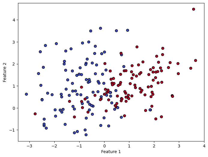
#3. 간단한 이진 분류 문제를 k-최근접이웃 알고리즘을 사용해 해결해보세요.

이진 분류에 대한 데이터셋이 제공 되지 않아 먼저 이진 분류 데이터셋 sklearn의 make_classification()메서드를 이용해 만들었다.

X, y = make_classification(n_samples=200, n_features=2, n_redundant=0,
                           n_informative=2, n_clusters_per_class=1, random_state=42)

만들어진 데이터셋을 시각화하여 어떤 형식인지 확인

plt.figure(figsize=(8, 6))
plt.scatter(X[:, 0], X[:, 1], c=y, cmap='coolwarm', edgecolors='k')
plt.xlabel('Feature 1')
plt.ylabel('Feature 2')
plt.show()

png

학습을 위해 train 데이터와 test 데이터를 분할 (8:2)

X_train, X_test, y_train, y_test = train_test_split(X, y, test_size=0.2, random_state=42)

print(f"train 데이터셋 개수 : {len(X_train)}, {len(y_train)}")
print(f"test 데이터셋 개수 : {len(X_test)}, {len(y_test)}")

train 데이터셋 개수 : 160, 160
test 데이터셋 개수 : 40, 40

KNN 모델 생성 및 학습

KNN = KNeighborsClassifier(n_neighbors=3)
KNN.fit(X_train, y_train)

KNeighborsClassifier(n_neighbors=3)

In a Jupyter environment, please rerun this cell to show the HTML representation or trust the notebook.
On GitHub, the HTML representation is unable to render, please try loading this page with nbviewer.org.

예측 수행 및 성능 평가

y_pred = KNN.predict(X_test)
confusion_matrix = metrics.confusion_matrix(y_test, y_pred)
accuracy = metrics.accuracy_score(y_test, y_pred)
precision = metrics.precision_score(y_test, y_pred)
recall = metrics.recall_score(y_test, y_pred)
f1 = metrics.f1_score(y_test, y_pred)

print(f"Confusion Matrix : \n{confusion_matrix}")
print(f"Accuracy : {accuracy}")
print(f"Precision : {precision}")
print(f"Recall : {recall}")
print(f"F1 Score : {f1}")

Confusion Matrix : 
[[22  1]
 [ 2 15]]
Accuracy : 0.925
Precision : 0.9375
Recall : 0.8823529411764706
F1 Score : 0.9090909090909091

#4. OR, NOT 연산을 모델링해보세요.

OR 모델링 (FastAPI 수업 내용 참고)

class Model_OR:

  def __init__(self):
    self.weights = np.random.rand(2)
    self.bias = np.random.rand(1)

  def step_function(self, x):
    return 1 if x >= 0 else 0

  def predict(self, x):
    z = np.dot(x, self.weights) + self.bias
    return self.step_function(z)

  def train(self):
    learning_rate = 0.1
    epochs = 20
    inputs = np.array([[0, 0], [0, 1], [1, 0], [1, 1]])
    outputs = np.array([0, 1, 1, 1])

    for epoch in range(epochs):
      for i in range(len(inputs)):
        total_input = np.dot(inputs[i], self.weights) + self.bias
        prediction = self.step_function(total_input)
        error = outputs[i] - prediction
        self.weights += learning_rate * error * inputs[i]
        self.bias += learning_rate * error

NOT 모델링</br> NOT 모델링은 1차원이므로 가중치와 가중치 업데이트를 스칼라로 변환

class Model_NOT:

  def __init__(self):
    self.weights = np.random.rand(1)
    self.bias = np.random.rand(1)

  def step_function(self, x):
    return 1 if x >= 0 else 0

  def predict(self, x):
    z = x * self.weights + self.bias
    return self.step_function(z)

  def train(self):
    learning_rate = 0.1
    epochs = 20
    inputs = np.array([0, 1])
    outputs = np.array([1, 0])

    for epoch in range(epochs):
      for i in range(len(inputs)):
        total_input = inputs[i] * self.weights + self.bias
        prediction = self.step_function(total_input)
        error = outputs[i] - prediction
        self.weights += learning_rate * error * inputs[i]
        self.bias += learning_rate * error

OR 모델 점검

orModel = Model_OR()
n = np.array([[0, 0], [0, 1], [1, 0], [1, 1]])

temp = []

for x in n:
  row = {
      '입력 1' : x[0],
      '입력 2' : x[1],
      '출력' : orModel.predict(x)
  }
  temp.append(row)

df = pd.DataFrame(temp)
print("OR 모델 학습 전:")
df

OR 모델 학습 후:

	입력 1	입력 2	출력
0	0	0	1
1	0	1	1
2	1	0	1
3	1	1	1

orModel.train()
temp = []

for x in n:
  row = {
      '입력 1' : x[0],
      '입력 2' : x[1],
      '출력' : orModel.predict(x)
  }
  temp.append(row)

df = pd.DataFrame(temp)
print("OR 모델 학습 후:")
df

OR 모델 학습 후:

	입력 1	입력 2	출력
0	0	0	0
1	0	1	1
2	1	0	1
3	1	1	1

NOT 모델 점검

notModel = Model_NOT()

temp = []
for x in [0, 1]:
  row = {
      '입력' : x,
      '출력' : notModel.predict(x)
  }
  temp.append(row)

df = pd.DataFrame(temp)
print("NOT 모델 학습 전:")
df

NOT 모델 학습 전:

	입력	출력
0	0	1
1	1	1

notModel.train()
temp = []

for x in [0, 1]:
  row = {
      '입력' : x,
      '출력' : notModel.predict(x)
  }
  temp.append(row)

df = pd.DataFrame(temp)
print("NOT 모델 학습 후:")
df

NOT 모델 학습 후:

	입력	출력
0	0	1
1	1	0

Twitter Facebook LinkedIn

4주차 과제

1. 가상의 학생 성적 데이터를 활용한 데이터 전처리 과정을 구현해보세요.

2. 가상 데이터셋을 생성한 뒤 데이터셋을 학습, 검증, 테스트 데이터셋으로 분할해보세요.

공유하기

참고

OnTheTop Service

Feature Map 기반 CNN 모델 최적화

Application Model

Natural Language Processing